基于比较的算法 复杂度O(N²)
我们讨论三种基于比较的算法:
- 冒泡
- 选择
- 插入
因为这些算法需要比较两个元素以决定是否交换位置,故称基于比较的算法。
这三种算法最容易实现,但不是最高效的。其时间复杂度是O(N²)。
冒泡算法
给定数组N个元素,冒泡算法会:
- 比较一对邻近的元素(a,b)。
- 当这对元素无序时,交换他们。(此是当a>b时)。
- 重复步骤1,步骤2直到数组尾。
- 此时,最大元素会是最后一个元素。然后令N=N-1,并重复步骤1直到N=1。
[29, 10, 14, 37, 14],冒泡的动画示意如下:
冒泡排序的分析
比较和交换需要常量时间,我们取c。
标准冒泡算法中有两层循环。
外层循环需要迭代N次。
但内层循环迭代的次数会越来越少:
- 当i=0, N-1次迭代 - 比较和(可能的)交换
- 当i=1,N-2次迭代
- 当i=2,N-3次迭代
… - 当N=N-2,1次迭代
- 当N=N-1,0次迭代
因此总共需要的迭代次数= (N-1) + (N-2) + ... + 1 + 0 = N*(N-1)/2。
总共花费的时间 = c * N*(N-1)/2 = O(N²)。
1 | |
冒泡改进 - 提前终止
冒泡排序并不高效,因为它是O(N²)的时间复杂度。
但若能提前终止(多余的)冒泡进程,时间复杂度可以提高到O(1)。
例:[3, 6, 11, 25, 39]。改进方法很简单:若内层循环没有发生交换,那么整个序列已经是正序的,此时可以终止冒泡进程。
讨论:这个改进让冒泡排序在一般情况下更快了,但无法改变其时间复杂度O(N²)的时间,为啥?
选择排序
令数组大小为N,L=0,选择排序步骤如下:
- 找到元素[L .. N-1]中最小元素X的位置。
- 将X元素和位置L的元素交换。
- L++,并重复步骤1。
1 | |
当然,也可以更改算法为找最大数并交换。
时间复杂度和冒泡是一样的O(N²)。
插入排序
插入排序有点像给手上的扑克牌排序的过程。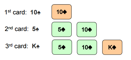
- 手上拿第一张牌。
- 拿到下一张牌,在目前有序的牌中找到正确的位置并插入新牌。
- 重复上述步骤直到所有牌结束。
1 | |
1 | |
分析插入排序
外层循坏需要N-1次迭代。
但内层循环的次数:
- 最好的情况下,只需要一次比较
a[j] > x就能确定是正序的,因此是O(1)。 - 最坏的情况下,数组是逆序的,这样每次迭代
a[j] > x都是true,每次都需要迭代整个内层循环,时间复杂度是O(N)。
因此,最好情况是O(1),最坏情况是O(N²)。
基于比较的 O(N log N) 的排序
- 归并排序
- 快速排序 和 随机快速排序
这些算法通常使用递归实现,采用分治思想, 归并排序和随机快速排序都是O(N log N)。
快速排序的非随机版本是O(N²)的。
归并排序
令数组大小为N,归并排序步骤如下:
- 将两个元素合并到一个正序的(仅含这两个元素)数组中。
- 将两个上述数组合并到一个正序的(现在含有四个元素)数组中。
- 最终:将两个各含有N/2的数组合并到一个数组中,则数组正序。
这仅是一个概要,我们还需要讨论更多细节才能应用归并排序
归并排序中复杂度O(N)的子步骤
我们将归并排序拆开讨论,先讨论复杂度为O(N)的子步骤。
令数组A大小为N1,数组B大小为N2,我们很容易将之合并为一个正序的大小N=N1+N2的数组
只需要比较数组的第一个元素,将较小的数组元素全部放到另一个数组之前。这个O(N)的操作需要额外的数组来存储数据。
1 | |
Golang实现:
1 | |
分治思想
分治法 - Divide and Conquer简写作D&C。
- Divide step:将一个问题分解成小的问题,然后递归的解决小的问题。
- Conquer step:将解决了的小问题合并起来,还原为原始问题的解。
归并算法的分治思想
归并算法是分治的一个应用。
divide step:将数组分为两半,然后递归的对两个数组分派归并排序。
conquer step:将结果集合并成解,这一步骤的工作量最大。
1 | |
Golang实现:
1 | |
归并排序时间复杂度分析
归并排序中merge的复杂度是O(N)的,那么merge执行的次数决定了最终的时间复杂度。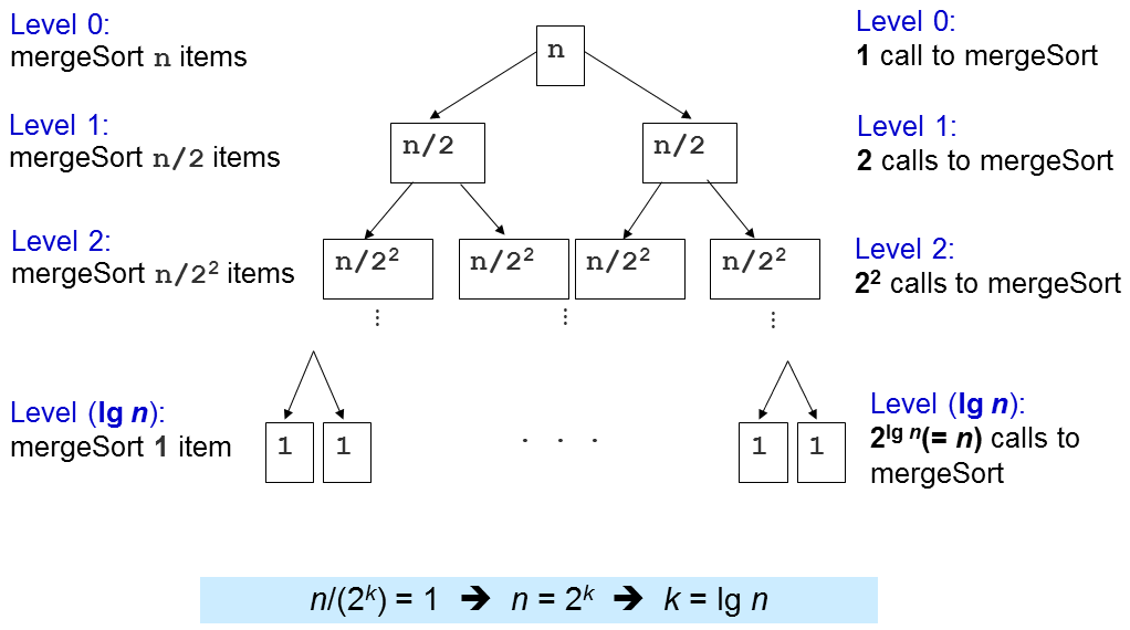
可以看到k=lg N,忽略常数,我们记归并排序的时间复杂度为O(N log N)。
归并排序的优缺点
首先,最重要的一点是,归并排序的时间复杂度稳定的是O(N log N),不受数据源的影响。没有任何的测试用例,不论数据源的大小,都不能是归并排序的时间超过O(N log N)。
目前为止,我们讨论过的算法中,归并排序是最适合处理大规模数据的算法。
当然,归并排序也有其劣势。
- 从头开始实现归并排序并不是很容易。
- 在合并阶段,需要额外的存储空间。因此内存利用率不高,也不是原地排序算法。
快速排序算法
快速排序也是分治法的应用。
Divide step:选择一个元素p,即pivot。
将数组a[i..j]分为三个部分:a[i..m-1], a[m], a[m=1..j]。
a[i..m-1]包含比p小的元素。
a[m]即pivot,m是p在数据源a中的索引。
a[m+1..j]包含了大于等于p的元素。
然后递归的重复上述步骤。
Conquer step:额,啥也不用做…
与归并排序对比,你会发现它的D&C步骤刚好相反。
分析快速排序
还是查分开讨论,先讨论复杂度为O(N)的子步骤。
为了分割a[i..j],我们先找到一个pivotp = a[i]。
剩下的a[i+1..j]将被分割为三个部分:
- S1=a[i+1..m],元素都 < P。
- S2=a[m+1..k-1],元素都 ≥ p。
- 未知部分 = a[k..j],其他元素待分配到S1 或 S2。
讨论:为什么选择p=a[i],有没有其他选择?
硬核讨论:若每次都将==p的元素放在S2里合适吗?
起初,S1和S2都是空的,所有的元素除了p=pivot都在未知区域中。
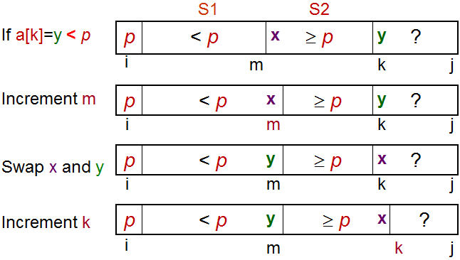
对于每一个在位置区域的元素a[k],将a[k]与p比较:
- a[k] ≥ p,将a[k]放入S2。
- a[k] < p,将a[k]放入S1。
最后交换a[i]和a[m],即将p放在S1和S2的中间。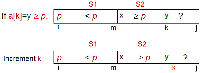
代码如下:1
2
3
4
5
6
7
8
9
10
11
12
13
14
15
16
17
18
19
20
21
22int partition(int a[], int i, int j) {
int p = a[i]; // p is the pivot
int m = i; // S1 and S2 are initially empty
for (int k = i+1; k <= j; k++) { // explore the unknown region
if (a[k] < p) { // case 2
m++;
swap(a[k], a[m]); // C++ STL algorithm std::swap
} // notice that we do nothing in case 1: a[k] >= p
}
swap(a[i], a[m]); // final step, swap pivot with a[m]
return m; // return the index of pivot
}
void quickSort(int a[], int low, int high) {
if (low < high) {
int m = partition(a, low, high); // O(N)
// a[low..high] ~> a[low..m–1], pivot, a[m+1..high]
quickSort(a, low, m-1); // recursively sort left subarray
// a[m] = pivot is already sorted after partition
quickSort(a, m+1, high); // then sort right subarray
}
}
Golang实现:
1 | |
快速排序的时间复杂度分析
partition操作只有一个循环,复杂度是O(N)。
那么快速排序的时间复杂度取决于partition执行的次数。
最坏情况下,当数据源是升序的,经过一轮后,S1是空的,S2包含除了pivot外其他元素。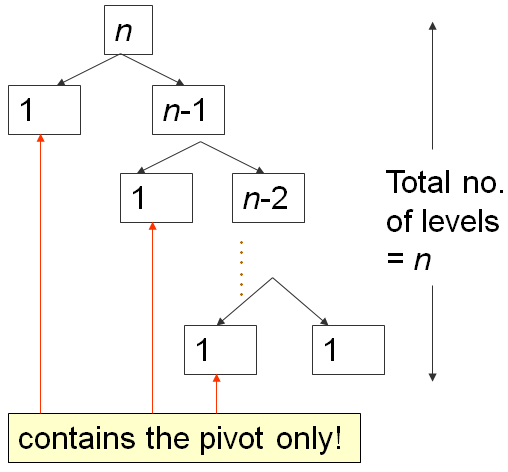
一共需要N轮循环,所以时间复杂度是O(N²)。
而最好情况下,每一次pivot都将数据源分割为两半,一共需要log N次。
因此复杂度是O(N log N)。
随机快速排序 - O(N log N)
It will take about 1 hour lecture to properly explain why this randomized version of Quick Sort has expected time complexity of O(N log N) on any input array of N elements.
In this e-Lecture, we will assume that it is true.
If you need non formal explanation: Just imagine that on randomized version of Quick Sort that randomizes the pivot selection, we will not always get extremely bad split of 0 (empty), 1 (pivot), and N-1 other items. This combination of lucky (half-pivot-half), somewhat lucky, somewhat unlucky, and extremely unlucky (empty, pivot, the rest) yields an average time complexity of O(N log N).
Discussion: Actually the phrase “any input array” above is not fully true. There is actually a way to make the randomized version of Quick Sort as currently presented in this VisuAlgo page still runs in O(N2). How?